---
title: "Solving Stochastic Differential Equations (SDE) in R with diffeqr"
author: "Chris Rackauckas"
date: "`r Sys.Date()`"
output: rmarkdown::html_vignette
vignette: >
%\VignetteIndexEntry{Solving Stochastic Differential Equations (SDE) in R with diffeqr}
%\VignetteEngine{knitr::rmarkdown}
%\VignetteEncoding{UTF-8}
---
```{r setup, include = FALSE}
knitr::opts_chunk$set(
collapse = TRUE,
comment = "#>"
)
```
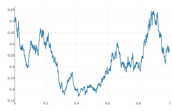
### 1D SDEs
Solving stochastic differential equations (SDEs) is the similar to ODEs. To solve an SDE, you use `diffeqr::sde.solve` and give
two functions: `f` and `g`, where `du = f(u,t)dt + g(u,t)dW_t`
```r
de <- diffeqr::diffeq_setup()
f <- function(u,p,t) {
return(1.01*u)
}
g <- function(u,p,t) {
return(0.87*u)
}
u0 <- 1/2
tspan <- list(0.0,1.0)
prob <- de$SDEProblem(f,g,u0,tspan)
sol <- de$solve(prob)
udf <- as.data.frame(t(sapply(sol$u,identity)))
plotly::plot_ly(udf, x = sol$t, y = sol$u, type = 'scatter', mode = 'lines')
```
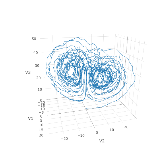
### Systems of Diagonal Noise SDEs
Let's add diagonal multiplicative noise to the Lorenz attractor. diffeqr defaults to diagonal noise when a system of
equations is given. This is a unique noise term per system variable. Thus we generalize our previous functions as
follows:
```R
f <- function(u,p,t) {
du1 = p[1]*(u[2]-u[1])
du2 = u[1]*(p[2]-u[3]) - u[2]
du3 = u[1]*u[2] - p[3]*u[3]
return(c(du1,du2,du3))
}
g <- function(u,p,t) {
return(c(0.3*u[1],0.3*u[2],0.3*u[3]))
}
u0 <- c(1.0,0.0,0.0)
tspan <- c(0.0,1.0)
p <- c(10.0,28.0,8/3)
prob <- de$SDEProblem(f,g,u0,tspan,p)
sol <- de$solve(prob,saveat=0.005)
udf <- as.data.frame(t(sapply(sol$u,identity)))
plotly::plot_ly(udf, x = ~V1, y = ~V2, z = ~V3, type = 'scatter3d', mode = 'lines')
```
Using a JIT compiled function for the drift and diffusion functions can greatly enhance the speed here.
With the speed increase we can comfortably solve over long time spans:
```R
tspan <- c(0.0,100.0)
prob <- de$SDEProblem(f,g,u0,tspan,p)
fastprob <- diffeqr::jitoptimize_sde(de,prob)
sol <- de$solve(fastprob,saveat=0.005)
udf <- as.data.frame(t(sapply(sol$u,identity)))
plotly::plot_ly(udf, x = ~V1, y = ~V2, z = ~V3, type = 'scatter3d', mode = 'lines')
```
Let's see how much faster the JIT-compiled version was:
```R
> system.time({ for (i in 1:5){ de$solve(prob ) }})
user system elapsed
146.40 0.75 147.22
> system.time({ for (i in 1:5){ de$solve(fastprob) }})
user system elapsed
1.07 0.10 1.17
```
Holy Monster's Inc. that's about 145x faster.
### Systems of SDEs with Non-Diagonal Noise
In many cases you may want to share noise terms across the system. This is known as non-diagonal noise. The
[DifferentialEquations.jl SDE Tutorial](https://diffeq.sciml.ai/dev/tutorials/sde_example/#Example-4:-Systems-of-SDEs-with-Non-Diagonal-Noise-1)
explains how the matrix form of the diffusion term corresponds to the summation style of multiple Wiener processes. Essentially,
the row corresponds to which system the term is applied to, and the column is which noise term. So `du[i,j]` is the amount of
noise due to the `j`th Wiener process that's applied to `u[i]`. We solve the Lorenz system with correlated noise as follows:
```R
f <- JuliaCall::julia_eval("
function f(du,u,p,t)
du[1] = 10.0*(u[2]-u[1])
du[2] = u[1]*(28.0-u[3]) - u[2]
du[3] = u[1]*u[2] - (8/3)*u[3]
end")
g <- JuliaCall::julia_eval("
function g(du,u,p,t)
du[1,1] = 0.3u[1]
du[2,1] = 0.6u[1]
du[3,1] = 0.2u[1]
du[1,2] = 1.2u[2]
du[2,2] = 0.2u[2]
du[3,2] = 0.3u[2]
end")
u0 <- c(1.0,0.0,0.0)
tspan <- c(0.0,100.0)
noise_rate_prototype <- matrix(c(0.0,0.0,0.0,0.0,0.0,0.0), nrow = 3, ncol = 2)
JuliaCall::julia_assign("u0", u0)
JuliaCall::julia_assign("tspan", tspan)
JuliaCall::julia_assign("noise_rate_prototype", noise_rate_prototype)
prob <- JuliaCall::julia_eval("SDEProblem(f, g, u0, tspan, p, noise_rate_prototype=noise_rate_prototype)")
sol <- de$solve(prob)
udf <- as.data.frame(t(sapply(sol$u,identity)))
plotly::plot_ly(udf, x = ~V1, y = ~V2, z = ~V3, type = 'scatter3d', mode = 'lines')
```
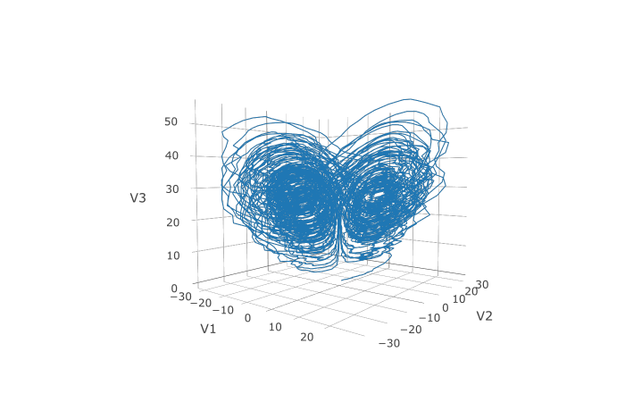
Here you can see that the warping effect of the noise correlations is quite visible!
Note that we applied JIT compilation since it's quite necessary for any difficult
stochastic example.